DFT introduction #2
Team Rutgers(Michele, Ezekiel & Valeria)Rutgers University-Newark |
 |
| An interactive session |
Retrieve this presentation at:
mini ASESMA 2026 \(\bullet\) Accra, Ghana \(\bullet\) June 17, 2026
Goal of this lecture#
Understand what basis sets are
Introduce basics about basis sets (PWs and local orbitals like GTOs)
Discretize the KS equations so they can be solved by a computer
Focus on PW (GTOs done on your own, numerical orbitals introduced by Javier later)
Split into N groups#
Assign number
1-Nto each studentGroups sit together
Possibly have 1 instructor per group
from IPython.display import IFrame
import numpy as np
import matplotlib.pyplot as plt
from ase.build import molecule
My assumptions#
Basic linear algebra (vectors, matrices, operators, wavefunctions)
Undergraduate QM
Dirac notation (i.e., i-th vector \(\to |i\rangle\) or \(|\psi_i\rangle\), scalar product between i and j \(\to \langle \psi_i | \psi_j\rangle\))
Kohn-Sham equations
Why are basis sets needed?#
They provide a representation
Allow us to discretize the problem
Let’s expand a function in a basis#
\(\{\chi_i(r)\}\) are basis functions forming a basis set
\(\{C_{ik}\}\) are expansion coefficients, \(C_{ik}\in \mathbb{C}\)
Examples of basis sets#
Plane waves (PW)
Gaussian-Type Orbitals (GTOs)
Numerical Orbitals (Javier will introduce later this week)
…
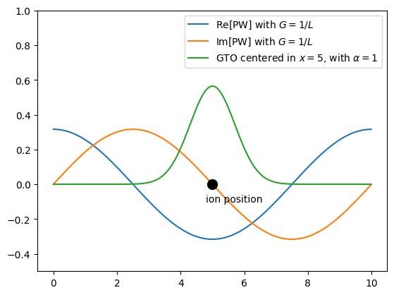
What do they look like? Let’s use Python#
L=10; X = np.linspace(start=0,stop=L,num=1000,endpoint=False)
def pw(x,G):
    return 1.0/np.sqrt(L)*np.exp(1j*2*np.pi*G*x)
def gto(x,center,alpha):
    return np.sqrt(alpha/np.pi)*np.exp(-alpha*(x-center)**2)
fig = plt.figure()#(figsize=(8,5))
plt.plot(X,np.real(pw(X,G=1/L)), label=r"Re[PW] with $G=1/L$")
plt.plot(X,np.imag(pw(X,G=1/L)), label=r"Im[PW] with $G=1/L$")
plt.plot(X,gto(X,center=5,alpha=1),label=r"GTO centered in $x=5$, with $\alpha=1$")
plt.plot(5, 0, 'ko', markersize=10); plt.text(x=4.8,y=-0.1,s="ion position")
plt.ylim([-.5,1]); plt.legend()
<matplotlib.legend.Legend at 0x13a53cdf0>
Challenge 1#
Are GTOs an orthonormal basis set? Justify.
Are PWs an orthonormal basis set? Justify.
The condition for orthonormality \(S_{ij}=\langle \chi_i | \chi_j\rangle = \delta_{ij}\).

How many plane waves are needed?#
You will attack this question in your Homework
The homework will introduce the
PW cutoffneeded by most PW codes, like QEFor QEpy, you will see something like (all values in Ry):
qe_options = {}
qe_options["&electrons"] = {}
qe_options["&electrons"]["ecutwf"] = 80
qe_options["&electrons"]["ecutrho"] = 320
ecutwfis the kinetic energy of the PW with the largest \(G\) point in Ryecutrhois the kinetic energy of the PW with the largest \(G\) point used to Fourier transform the electron density \(n(r)\) in RyLet me know during the break if you wish to know why these two cutoffs are different.
Challenge 1.2#
Convert 1 Ha into Ry
Convert 1 Ry into eV
How do basis sets “discretize” the KS equations?#
Working with your group mates, discretize the KS equations
Discretized KS equations#
The final result should be
or in matrix form
\(\mathbb{H}\): The KS Hamiltonian, mean field Hamiltonian or Fock matrix
\(\mathbb{C}\): The matrix of the coefficients. Each column represents a KS orbital. In PW, these are simply the
bands\(\varepsilon\): A diagonal matrix with the orbital energies, \(\varepsilon_k\). Also KS eigenvalues, …
\(\mathbb{S}\): Overlap matrix. Diagonal in PW.
Matrix elements of \(\hat T\) in plane waves, needed to solve \(\mathbb{HC=SC\varepsilon}\)#
Matrix elements of \(v_s(r)\), needed to solve \(\mathbb{HC=SC\varepsilon}\)#
But… we can use the \(G\) components of \(\tilde v_s(G)\):
which gives the matrix elements of \(v_s\) almost directly.
Hartree potential, the (computationally) most difficult piece of \(v_s(r)\)#
Challenge 2#
Can you derive the equations we just presented?
Now we can solve \(\mathbb{HC=C\varepsilon}\)?#
Remember \(v_s(r) = v_{eN}(r) + v_H(r) + v_{xc}(r)\).
First, a note on PWs#
Many plane waves are needed to represent “spiky” or highly oscillatory features, such as \(v_{eN}(r)\) and \(n(r)\) in the ionic core region.
Thus, pseudopotentials are typically employed to:
avoid the Coulomb singularity of the electron–nuclear interaction potential;
remove the need to represent the atomic cores, where densities and orbitals are highly oscillatory. More on this from Javier tomorrow!
Why are PW basis so useful?#
Orthonormal!
Systematically improvable: higher \(N\) (or equivalently \(\max\left[ G \right]\)) leads to better results.
Evaluation of the kinetic-energy operator and solution of the Poisson equation are easy, with \(\mathcal{O}(N\ln N)\) complexity.