Introduction to DFT and TDDFT

Set of lectures delivered at mini ASESMA 2026

Instructors

• Michele Pavanello

• Valeria Rios Vargas

• Ezekiel Oyeniyi

Affiliation

Pavanello Research Group

Department of Physics

Rutgers University-Newark

Aim

These lectures are for those graduate students in physics, chemistry and material science who wish to understand the basics of DFT and TDDFT. The focus is plane wave implementations with emphasis on the basics. For example, analyses of pseudopotentials and exchange-correlation functionals are not entartained.

Format

Each chapter is extracted form a Jupyter Notebook Rise presentation supporting a 1.5 hour lecture. Hands-on excercises are integral part of the lectures and can be carried out over the Google Collaboratory.

Homework

• Fourier Transformations. Go through this before lecture 2.

• Finding a good the plane wave cutoff. Go through this after lecture 2.

Hands on excercises. All use QEpy.

• Solving the Self-Consistent Field problem with QEpy

• Equation of State of Aluminum

• Relax the structure of a molecule

• Run a dynamics of the structure of a molecule

• Band structure of graphene

• TDDFT spectra of molecular systems and solids at the gamma point with aufbau occupations

DFT introduction #1

Team Rutgers (Valeria, Ezekiel and Michele)
	An interactive session

Retrieve this presentation at:

https://github.com/asesma-org/miniASESMA2026

mini ASESMA 2026 \(\bullet\) Accra, Ghana \(\bullet\) June 16, 2026

Goals of this lecture

• Reasons for considering DFT

• Basics of the theory behind DFT and Kohn-Sham DFT

• KS equations and XC functional

Split into N groups

• Assign number 1-N to each student

• Groups sit together

• Possibly have 1 instructor per group

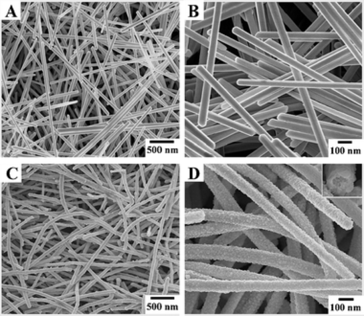
The Real World

Photocatalyst	Catalytic nanoparticles
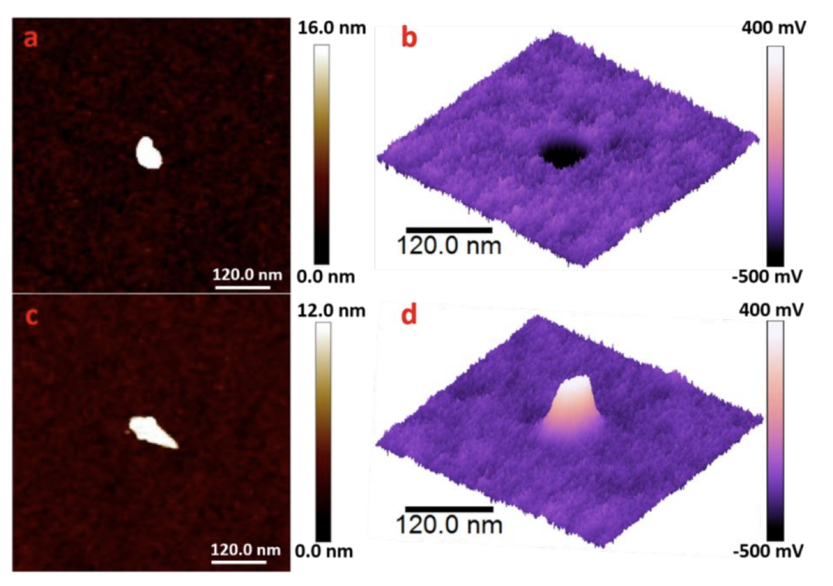Chem. Comm., 43, 6551 (2009)	PCCP, 21, 15080 (2019)

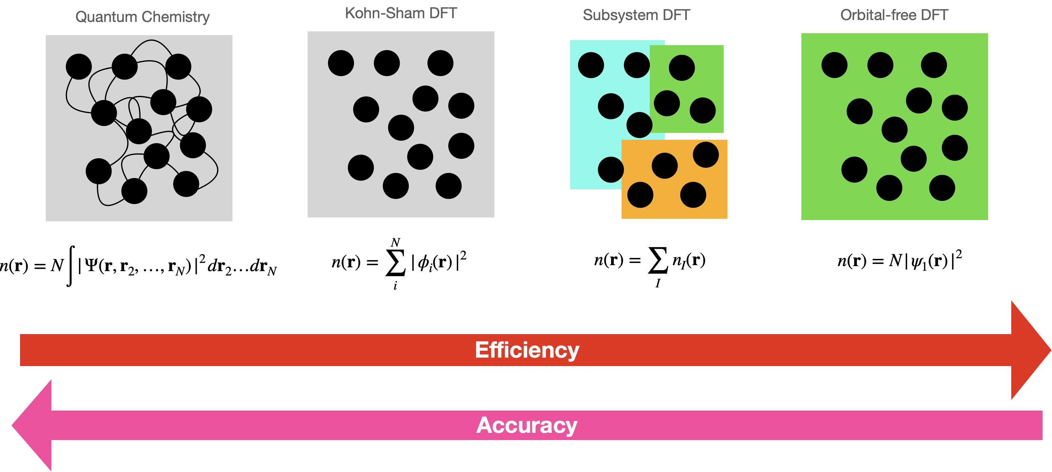
Available electronic structure methods

Challenge 1

Let’s check your QM knowledge.

• What is the molecular Hamiltonian?

Solution to Challenge #1 and a bit more…

Molecular Hamiltonian for interacting electrons and nuclei of charge \(Z_\alpha\)

\[ \hat{H} = \underbrace{-\frac{1}{2}\sum_i^{N_e} \nabla^2_i}_{\hat T} + \underbrace{\sum_i^{N_e}\sum_\alpha^{N_n} \frac{-Z_\alpha}{|r_i-R_\alpha|}}_{\hat V_{eN}} + \underbrace{\frac{1}{2}\sum_{i\neq j}^{N_e} \frac{1}{|r_i-r_j|}}_{\hat V_{ee}} + E_{NN} \]

The Schrödinger equation for the ground state of the interacting system

\[ \hat H \Psi_0 = E_0 \Psi_0 \]

Expectation values of each term of the Hamiltonian

\[ T[\Psi_0] = \langle \Psi_0 | \hat T | \Psi_0 \rangle, ~~ E_{ee}[\Psi_0] = \langle \Psi_0 | \hat V_{ee} | \Psi_0 \rangle \]

\[ E_{eN}[\Psi_0] = \color{red}{E_{eN}[n]} = \langle \Psi_0 | \hat V_{eN} | \Psi_0 \rangle = \int n(r) v_{eN}(r) dr \]

The Hohenberg and Kohn theorems

\[ \Psi_0 \longleftrightarrow n(r) \longleftrightarrow v_{eN}(r) \longleftrightarrow \Psi_0 \]

Therefore \(n(r)\), \(v_{eN}(r)\) or \(\Psi_0\) hold the same information.

HK paper 1964

In particular:

\[ E \equiv E[\Psi_0] \equiv E[v_{eN}] \equiv E[n] \]

DFT exploits the latter as follows:

$$ E[n] = T[n] + E_{ee}[n]+E_{eN}[n]+E_{NN} $$

Challenge 2

What do the energy functionals mean?

• Write an expression for each of the functionals (\(T\), \(E_{ee}\), \(E_{eN}\)) in terms of \(n(r)\) and/or of \(\Psi_0\).

Solution to Challenge #2 and a bit more…

Recalling:

\[ \color{red}{E_{eN}[n]} = \langle \Psi_0 | \hat V_{eN} | \Psi_0 \rangle = \int n(r)\,v_{eN}(r)\,dr \]

Because \(v_{eN}\) is fixed by the system's geometry, \(E_{eN}\) is already a density functional.

For the other terms in the Hamiltonian:


$\( T[\Psi_0] = \langle \Psi_0 | \hat T | \Psi_0 \rangle, ~~ E_{ee}[\Psi_0] = \langle \Psi_0 | \hat V_{ee} | \Psi_0 \rangle \)$

Apparently, \(T\) and \(E_{ee}\) cannot be written as denisty functionals...

What can we do with the HK theorems?

\(n(r)\)

...the density determines everything... in principle.... but is this useful? ... Are the functionals involved known?

Introducing: the Kohn-Sham (KS) system of noninteracting electrons

KS paper 1965

The density of the KS system is the same as the interacting system.

\[ v_s(r) \longleftrightarrow n(r) \longleftrightarrow v_{eN}(r) \]

Energy functional for the KS system

\[ E[n] = \color{red}{T[n] + E_{ee}[n]}+E_{eN}[n]+E_{NN} \]

\[E[n] = \color{red}{T_s[n] + E_{H}[n] + E_{xc}[n]}+ E_{eN}[n]+ E_{NN}\]
where the density $n(r) = \sum_i^N |\phi_i(r)|^2$.

The KS kinetic energy is

\[ T_{s}[n] \equiv T_s[\{\phi_i\}]= -\frac{1}{2}\sum_i \langle \phi_i | \nabla^2 | \phi_i\rangle = -\frac{1}{2}\sum_i \int \phi_i^*(r) \nabla^2 \phi_i(r) dr \]

Mind: \(T_s \neq T\).

The classical e-e repulsion (Hartree) and e-N attraction:

\[ E_H[n]=\frac{1}{2}\int \frac{n(r)n(r')}{|r-r'|}drdr' \qquad\qquad E_{eN}[n] = \int n(r) v_{eN}(r) dr \]

Challenge 3: What is \(E_{xc}\)?

Derive an expression for \(E_{xc}\)

• Derive an expression for \(E_{xc}\) in terms of \(T\), \(E_{ee}\), \(T_s\) and \(E_H\).

Solution to Challenge #3

The energy functional, whether KS or interacting, should yield the same energy value, therefore

\[ E_{xc}[n] = E_{ee}[n]-E_H[n] + T[n]-T_s[n] \]

Can \(E_{xc}[n]\) be approximated?

Usually it is approached by separating exchange, \(E_x\), and correlation, \(E_c\): \[ E_{xc}[n] = E_x[n] + E_c[n] \]

Local Density Approximation from the UEG. Example from Dirac's exchange: \[ E_{x}^{\rm UEG} = - c_x \bar n^{4/3} V \longrightarrow E_x[n] \simeq -c_x \int n^{4/3}(r) dr \]

• QEpy uses same structure as QE to specify the xc functional

qe_options = {}
qe_options["&system"] = {}
qe_options["&system"]["input_dft"] = 'LDA'

• Typically xc is already specified in the pseudopotential files.

Solving for the electronic structure (find the KS orbitals, \(\{\phi_i\}\))

To minimize the energy, we define an appropriate Lagrangian:

\[ \mathcal{L}_{KS}[\{\phi_i\}] = E[\{\phi_i\}] - \sum_{ij} \varepsilon_{ij}\left(\langle \phi_j|\phi_i \rangle - \delta_{ij}\right) \]

At the minimum, we impose \(\frac{\delta \mathcal{L}_{KS}[\{\phi_i\}]}{\delta \langle \phi_j|}=0\) or just \(\frac{\delta \mathcal{L}_{KS}[\{\phi_i\}]}{\delta \phi_j^*(r)}=0\), and choose the so-called canonical orbitals (i.e., \(\varepsilon_{ij}=\varepsilon_{i}\delta_{ij}\)).

This yields the Kohn-Sham equations:

\[ -\frac{1}{2}\nabla^2 \phi_i(r) + v_s[n](r)\phi_i(r) = \varepsilon_i\phi_i(r) \]

where \(v_s(r)\) includes effects of e-N attraction and e-e repulsion. But what is \(v_s(r)\)?

Challenge 4

Considering the chain rule of functional differentiation (\(\phi^*\) and \(\phi\) are considered independent variables):

\[ \frac{\delta F[n]}{\delta \phi_j^*(r)} = \int \frac{\delta F[n]}{\delta n(r')} \frac{\delta n(r')}{\delta \phi_j^*(r)} \,dr' = \frac{\delta F[n]}{\delta n(r)}\phi_j(r). \]

Show that the KS potential is given by:

\[\begin{split} \color{green}{ \begin{aligned} v_s[n](r) &= \frac{\delta E_H[n]}{\delta n(r)} + \frac{\delta E_{xc}[n]}{\delta n(r)} + v_{eN}(r) \\[0.5em] &= \int \frac{n(r')}{|r-r'|} \,dr' + \frac{\delta E_{xc}[n]}{\delta n(r)} + v_{eN}(r). \end{aligned} } \end{split}\]

Can you derive the KS equations?

DFT introduction #2

Team Rutgers (Michele, Ezekiel & Valeria) Rutgers University-Newark
	An interactive session

Retrieve this presentation at:

https://github.com/asesma-org/miniASESMA2026

mini ASESMA 2026 \(\bullet\) Accra, Ghana \(\bullet\) June 17, 2026

Goal of this lecture

• Understand what basis sets are

• Introduce basics about basis sets (PWs and local orbitals like GTOs)

• Discretize the KS equations so they can be solved by a computer

• Focus on PW (GTOs done on your own, numerical orbitals introduced by Javier later)

Split into N groups

• Assign number 1-N to each student

• Groups sit together

• Possibly have 1 instructor per group

from IPython.display import IFrame
import numpy as np
import matplotlib.pyplot as plt
from ase.build import molecule

My assumptions

• Basic linear algebra (vectors, matrices, operators, wavefunctions)

• Undergraduate QM

• Dirac notation (i.e., i-th vector \(\to |i\rangle\) or \(|\psi_i\rangle\), scalar product between i and j \(\to \langle \psi_i | \psi_j\rangle\))

• Kohn-Sham equations

Why are basis sets needed?

• They provide a representation

• Allow us to discretize the problem

Let’s expand a function in a basis

\[ \psi_k(r) = \sum_i C_{ik} \chi_i(r) \]

• \(\{\chi_i(r)\}\) are basis functions forming a basis set

• \(\{C_{ik}\}\) are expansion coefficients, \(C_{ik}\in \mathbb{C}\)

Examples of basis sets

• Plane waves (PW)

\[ \chi_{G}(r) = \frac{1}{\sqrt{\Omega}} e^{iGr} \]

• Gaussian-Type Orbitals (GTOs)

\[ \chi_{\mu,\alpha}(r) = \left(\frac{2\alpha}{\pi}\right)^{d/2} e^{-\alpha |r-\mu|^2} \]

• Numerical Orbitals (Javier will introduce later this week)

• …

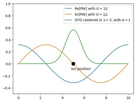
What do they look like? Let’s use Python

L=10; X = np.linspace(start=0,stop=L,num=1000,endpoint=False)
def pw(x,G):
    return 1.0/np.sqrt(L)*np.exp(1j*2*np.pi*G*x)
def gto(x,center,alpha):
    return np.sqrt(alpha/np.pi)*np.exp(-alpha*(x-center)**2)

fig = plt.figure()#(figsize=(8,5))
plt.plot(X,np.real(pw(X,G=1/L)), label=r"Re[PW] with $G=1/L$")
plt.plot(X,np.imag(pw(X,G=1/L)), label=r"Im[PW] with $G=1/L$")
plt.plot(X,gto(X,center=5,alpha=1),label=r"GTO centered in $x=5$, with $\alpha=1$")
plt.plot(5, 0, 'ko', markersize=10); plt.text(x=4.8,y=-0.1,s="ion position")
plt.ylim([-.5,1]); plt.legend()

<matplotlib.legend.Legend at 0x13a53cdf0>

Challenge 1

• Are GTOs an orthonormal basis set? Justify.

• Are PWs an orthonormal basis set? Justify.

The condition for orthonormality \(S_{ij}=\langle \chi_i | \chi_j\rangle = \delta_{ij}\).

How many plane waves are needed?

• You will attack this question in your Homework

• The homework will introduce the PW cutoff needed by most PW codes, like QE

• For QEpy, you will see something like (all values in Ry):

qe_options = {}
qe_options["&electrons"] = {}
qe_options["&electrons"]["ecutwf"] = 80
qe_options["&electrons"]["ecutrho"] = 320

• ecutwf is the kinetic energy of the PW with the largest \(G\) point in Ry

• ecutrho is the kinetic energy of the PW with the largest \(G\) point used to Fourier transform the electron density \(n(r)\) in Ry

• Let me know during the break if you wish to know why these two cutoffs are different.

Challenge 1.2

• Convert 1 Ha into Ry

• Convert 1 Ry into eV

How do basis sets “discretize” the KS equations?

Working with your group mates, discretize the KS equations

\[-\frac{1}{2}\nabla^2 \phi_k(r) + v_s(r) \phi_k(r) = \varepsilon_k \phi_k(r)\]

Use: \(\{\chi_i(r)\}\) such that \(\phi_k(r) = \sum_i C_{ik}\chi_i(r)\)

Consider: KS Hamiltonian matrix elements are \(H_{ji}=\langle \chi_j \mid \hat H \mid \chi_i \rangle\), and the overlap elements among the basis functions are \(S_{ji}=\langle \chi_j \mid \chi_i \rangle\).

Discretized KS equations

The final result should be

\[ \sum_i H_{ji}C_{ik} = \varepsilon_k \sum_i S_{ji} C_{ik} \]

or in matrix form

\[ \color{green}{\mathbb{H}\mathbb{C} = \mathbb{S}\mathbb{C}\boldsymbol{\varepsilon}} \]

• \(\mathbb{H}\): The KS Hamiltonian, mean field Hamiltonian or Fock matrix

• \(\mathbb{C}\): The matrix of the coefficients. Each column represents a KS orbital. In PW, these are simply the bands

• \(\varepsilon\): A diagonal matrix with the orbital energies, \(\varepsilon_k\). Also KS eigenvalues, …

• \(\mathbb{S}\): Overlap matrix. Diagonal in PW.

Matrix elements of \(\hat T\) in plane waves, needed to solve \(\mathbb{HC=SC\varepsilon}\)

\[ \langle \chi_i | \hat T | \chi_j \rangle = \left\langle \chi_i \left| -\frac{1}{2} \nabla^2 \right| \chi_j \right\rangle =-\frac{1}{2\Omega} \int dr ~ -G_j^2 ~ e^{i(G_j-G_i)}r = \mathbf{\color{red}{\frac{G_j^2}{2}\delta_{ij}}} \]

It's diagonal! ... and cheap to compute ...

Matrix elements of \(v_s(r)\), needed to solve \(\mathbb{HC=SC\varepsilon}\)

\[ \langle \chi_i | v_s | \chi_j\rangle = \frac{1}{\Omega}\int dr v_s(r) e^{i(G_j-G_i)r} \]

Not a diagonal matrix

But… we can use the \(G\) components of \(\tilde v_s(G)\):

\[ \langle \chi_i | v_s | \chi_j\rangle = \frac{1}{\Omega}\tilde v_s(G_j-G_i) \]

which gives the matrix elements of \(v_s\) almost directly.

Hartree potential, the (computationally) most difficult piece of \(v_s(r)\)

\[ v_H(r) = \int dr' \frac{n(r')}{|r-r'|} \equiv \color{red}{n \star \frac{1}{|r|}} \qquad \text{Poisson equation} \]

Let's use the convolution theorem : \(f = h \star g \;\longrightarrow\; \tilde f = \tilde h \cdot \tilde g\)

\[ \tilde v_H(G) = \tilde n(G) \frac{4\pi}{G^2} \to \langle \chi_i | v_H | \chi_j\rangle = \frac{1}{\Omega} \tilde v_H(G_j-G_i) \]

Thanks to Fast Fourier Transforms (FFT), the \(v_H\) potential is computed with \(\mathcal{O}(N\ln N)\) operations!

Challenge 2

• Can you derive the equations we just presented?

Now we can solve \(\mathbb{HC=C\varepsilon}\)?

\[\begin{split} H_{ij} = \left[ \frac{G_i^2}{2} \delta_{ij} + \frac{1}{\Omega}\tilde v_s(G_j - G_i) \right] \\ \text{ ... and ... } S_{ij} = \delta_{ij} \end{split}\]

Remember \(v_s(r) = v_{eN}(r) + v_H(r) + v_{xc}(r)\).

Is it enough?

\(v_H\) and \(v_{xc}\) depend on \(n(r)\). Do we know what \(n(r)\) is?

We'll get to this later

First, a note on PWs

• Many plane waves are needed to represent “spiky” or highly oscillatory features, such as \(v_{eN}(r)\) and \(n(r)\) in the ionic core region.

• Thus, pseudopotentials are typically employed to:

  1. avoid the Coulomb singularity of the electron–nuclear interaction potential;

  2. remove the need to represent the atomic cores, where densities and orbitals are highly oscillatory. More on this from Javier tomorrow!

Why are PW basis so useful?

• Orthonormal!

• Systematically improvable: higher \(N\) (or equivalently \(\max\left[ G \right]\)) leads to better results.

• Evaluation of the kinetic-energy operator and solution of the Poisson equation are easy, with \(\mathcal{O}(N\ln N)\) complexity.

Break time!

DFT introduction #3 (short lecture)

Team Rutgers (Michele, Ezekiel & Valeria) Rutgers University-Newark
	An interactive session

Retrieve this presentation at:

https://github.com/asesma-org/miniASESMA2026/

mini ASESMA 2026 \(\bullet\) Accra, Ghana \(\bullet\) June 17, 2026

Goal of this lecture

• Understand occupations (aufbau and smearing)

• Understand and code the Self-Consistent Cycle (SCF)

• Band structure / DOS

Split into N groups

• Assign number 1-N to each student

• Groups sit together

• Possibly have 1 instructor per group

The KS equations

\[-\frac{1}{2}\nabla^2 \phi_k(r) + v_s(r) \phi_k(r) = \varepsilon_k \phi_k(r)\]

In discretized form

\[ \color{green}{\mathbb{HC}=\mathbb{SC\varepsilon}} \]

How can we solve it?

Generalized eigenvalue problem

\(\mathbb{H}\) depends on \(v_s(r)\) which depends on \(n(r)\)

What \(n(r)\) should we use to evaluate \(\mathbb{H}\)?

• uniform density

• sum of atomic densities (SAD), usually taken from the pseudopotential

But this is only a guess...

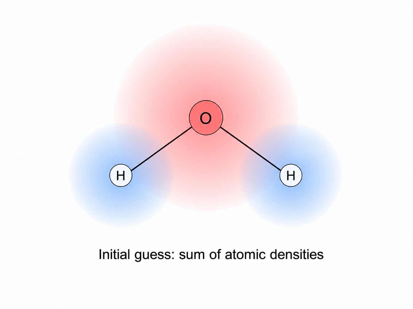
The Self-Consistent Field (SCF) loop

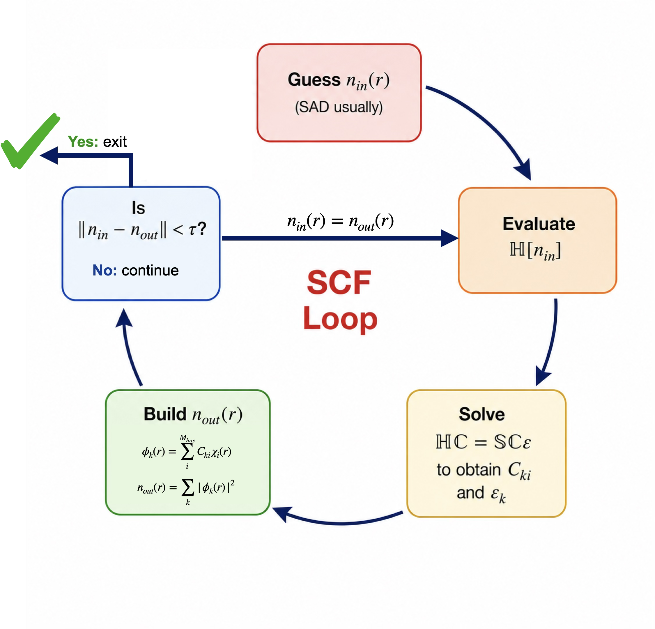
In QEpy and QE, the SCF is a basic workflow

• QE handles it via the card &control

• QEpy via the equivalent card in the options dictionary, like this:

qe_options = {}
qe_options['&control'] = {}
qe_options['&control']['calculation'] = 'scf'

The SCF threshold

\(\tau\) usually is in units of energy. Appropriate convergence conditions are

\[ \int \left|n_{\mathrm{in}}(r)-n_{\mathrm{out}}(r)\right|\,dr < \tau \]

\[ \int \frac{ \bigl(n_{\mathrm{out}}(r)-n_{\mathrm{in}}(r)\bigr) \bigl(n_{\mathrm{out}}(r')-n_{\mathrm{in}}(r')\bigr) }{ |r-r'| } \,dr\,dr' < \tau \]

\(\longrightarrow\) this is the condition adopted by QE

Challenge 1

• The electron density

Derive the equation for obtaining the electron density from the basis functions \(\{\chi_k(r)\}\) and the wavefunction coefficients \(\{C_{ki}\}\). Use the expression

\[ n(r) = \sum_k^N |\phi_k(r)|^2, \text{ assume for simplicity } \phi_k(r)\in \mathbb{R} \]

Occupation numbers

The usual equation (remember (N) is the number of electrons):

\[ n(r)=\sum_{k=1}^{N}\left|\phi_k(r)\right|^2 \qquad \longrightarrow \qquad \text{Aufbau occupations} \]

For nonzero \(T\), or for small gaps \(\left(E_g \ll 1\right)\), where the SCF procedure may have difficulty converging:

\[ n(r) = \sum_k f_k \left|\phi_k(r)\right|^2, \qquad \sum_k f_k = N \]

where \(f_k\) are called occupation numbers.

For solids, the need for (k)-point sampling often requires smearing:

\[ n(r) = \sum_k \sum_{\nu \in \mathrm{FBZ}} f_{k\nu}\left|\phi_{k\nu}(r)\right|^2, \qquad \sum_{k,\nu} f_{k\nu}=N \]

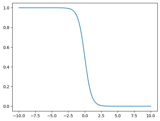
Challenge 2: what are these \(f_k\)?

• Code your own Fermi-Dirac smearing function to generate occupation numbers \(\{f_k\}\) given orbital energies \(\{\varepsilon_k\}\)

Consider a set of eigenvalues, \(\{\varepsilon_k\}\) coming from \(\color{green}{\mathbb{HC}=\mathbb{SC\varepsilon}}\). Evaluate the Fermi-Dirac distribution and impose \(\sum_k f_k = N\). Feel free to use AI to help you code it. Justify and explain your code to a tutor.

import matplotlib.pyplot as plt
import numpy as np
x=np.linspace(start=-10,stop=10,num=100)
tau = 0.5
plt.plot(x,(1+np.exp((x-0)/tau))**(-1))

[<matplotlib.lines.Line2D at 0x138595a50>]

Now time for hands-on activities: "SCF with QEpy" (and have QE solve it!)

Orbital energies and TDDFT

Some python code to run the example later...

import numpy as np
from qepy.calculator import QEpyCalculator
from ase.lattice.hexagonal import Graphene
from dftpy.formats import download_files
from ase import Atoms
import matplotlib.pyplot as plt
qe_options = {
    '&control': {
        'calculation': "'scf'",
        'prefix': "'tmp'",
        'pseudo_dir': "'./'"},
    '&system': {
        'ibrav' : 0,
        'ecutwfc': 20,
        'ecutrho': 200},
    '&electrons': {
        'conv_thr' : 1.0e-8},
     'atomic_species': ['C 12.0107 C.pz-vbc.UPF'],
     'k_points automatic': [' 9 9 1 0 0 0'],
}
additional_files = {
    'C.pz-vbc.UPF' : 'https://pseudopotentials.quantum-espresso.org/upf_files/C.pz-vbc.UPF',
}
download_files(additional_files)

Goals of this lecture + hands-on session

Part I

• The meaning and usefulness of DFT orbitals and orbital energies

• Band structure with QEpy

Part II

• Basic theory of KS TDDFT (real-time and linear response)

• Linear-response KS TDDFT

• Real-time KS TDDFT

Part III

• Hands on: LR-TDDFT simulations of molecules with QEpy

PART I: KS orbitals

What is the physical meaning of KS orbitals?

• Generally KS or HF orbitals have no rigorous physical meaning

• The HOMO is different: HF has Koopmans’ theorem and KS has Janak’s theorem relating it to the IP.

• What about the virtuals? The LUMO? … no rigorous physical meaning.

An overview of what you can do with orbitals

Yes! In a few ways.

If you are interested in ionization energies:

• GW

\[ \varepsilon_i \to \varepsilon_i + \langle \phi_i | \hat \Sigma(\varepsilon_i) - v_{xc} | \phi_i \rangle \]

• GW quasiparticle energies provide rigorous ionizations / affinities

• Hybrid functionals in DFT (HSE, PBE0, …) approximate GW results and usually predict ionizations/affinities via orbital energies much better than GGA functionals, like PBE

If you are interested in excitation energies:

• TDDFT

\[ \varepsilon_a-\varepsilon_i \to (\varepsilon_a-\varepsilon_i) + \left\langle \phi_i\phi_a \bigg| \frac{1}{|r-r'|}+f_{xc}(r,r',\varepsilon_a-\varepsilon_i) \bigg| \phi_i\phi_a \right\rangle+\cdots \]

where \(i,j,k,l,\ldots \in \text{occupied}\) and \(a,b,c,d,\ldots \in \text{virtuals}\).

Check out this paper by Baerends about the quality of KS virtuals vs HF virtuals for describing excitation energies

Comparing calculated and measured electronic energies

Photoemission (PES / XPES) and DFT orbital energies

• Photoemission spectroscopy (PES) ejects electrons with a photon and reports \(h\nu-E_{kin}\).

• With LDA or GGA functionals (e.g. PBE), orbital energies and gaps are not quantitatively accurate.

• Hybrid functionals and GW are used when agreement with PES/XPS matters.

Band structure: ARPES vs theory (graphene)

• Angle-resolved photoemission (ARPES) maps occupied bands \(E_n(\mathbf{k})\) in momentum space.

• A classic example is monolayer graphene on SiC: Bostwick et al., Nature Physics 3, 36 (2007).

• Panel (a): ARPES overlaid with a DFT calculation.

• The linear Dirac cones at \(K\) are reproduced.

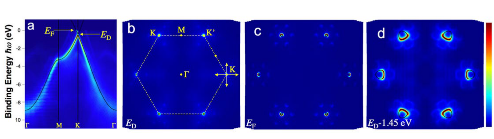
Figure adapted from Bostwick et al., Nature Physics 3, 36 (2007), Fig. 1.

Challenge 1

• In the limit of having the exact exchange-correlation functional, should you expect KS-DFT orbital energies to deliver exact band structures?

• Discuss among the group and be ready to share your thoughts with the class.

Band structures: Graphene

Build system and solve SCF

atoms = Graphene('C', latticeconstant={'a':2.46, 'c': 7})
atoms.calc = QEpyCalculator(qe_options=qe_options, logfile='tmp.out')
energy = atoms.get_potential_energy()

Look at the FBZ and select special \(k\) points

lat = atoms.cell.get_bravais_lattice()
lat.plot_bz(show=True)

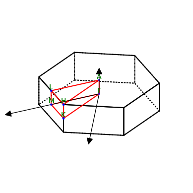
<Axes3D: >

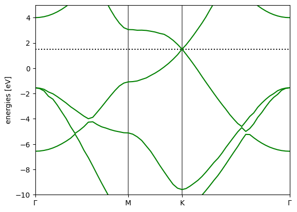
Choose \(\Gamma \to M \to K \to \Gamma\) band path

Plot the first 6 bands

path = atoms.cell.bandpath('GMKG',npoints=61)
qe_options['&system']['nbnd']=8
band = atoms.calc.get_band_structure(qe_options, kpts=path)#, reference=atoms.calc.get_fermi_level())
band.subtract_reference()
band.plot()

<Axes: ylabel='energies [eV]'>

Challenge 1.2

• Band structure of Si diamond structure

• Use the hands-on band structure tutorial. Notice the ASE tool Bulk from ase.build

from ase.build import bulk
atoms = bulk('Si','diamond',a=5.431)

• Compare the notebook for Si and for graphene

• Make a new notebook with a system of your choice and compute the band structure.

PART II: TDDFT based on KS-DFT

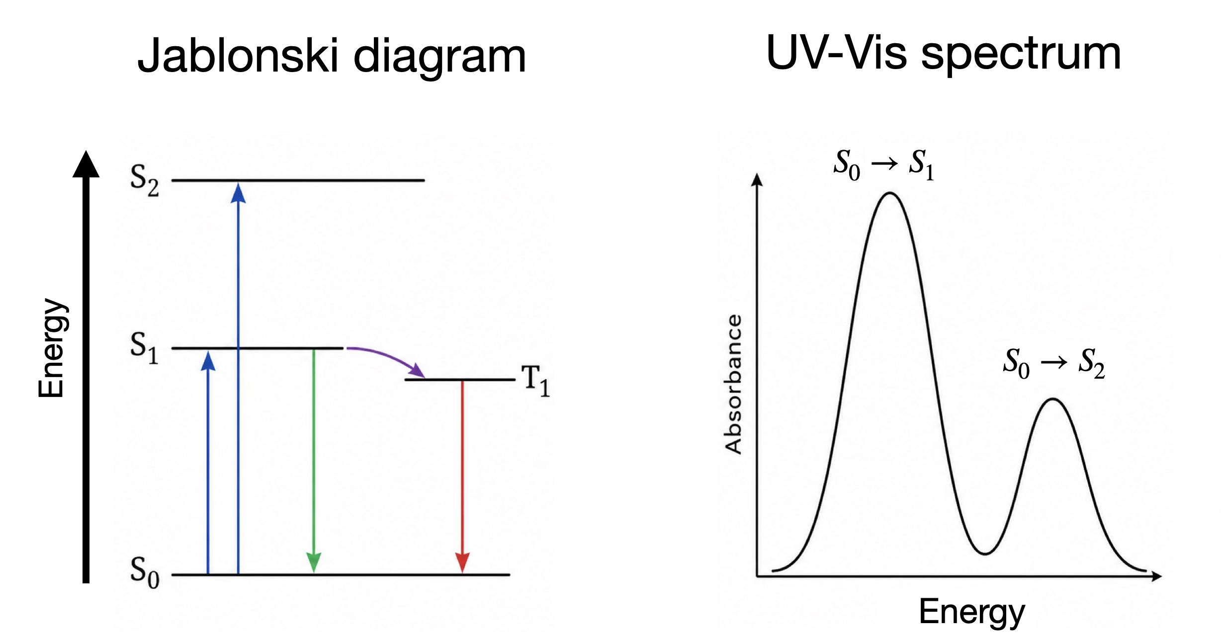
Electronic excitations and UV–vis spectroscopy

• UV–vis absorption probes electronic excitations from the ground singlet \(S_0\) to excited singlets \(S_n\) at photon energy \(E = h\nu\).

• In a Jablonski diagram, upward arrows are absorption; downward arrows are fluorescence; wavy/dashed paths are internal conversion and intersystem crossing.

• Each allowed \(S_0 \to S_n\) transition contributes a peak in the spectrum.
  
  

TDDFT vs experiment: \(S_0 \to S_1\) excitation energies

• Benchmark on 29 small molecules: mean absolute error (MAE) of \(S_0 \to S_1\) excitations vs experiment.

• Wavefunction methods vs TD-DFT functionals.
  
  

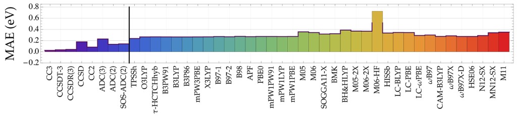
Adapted from Suellen et al., J. Chem. Theory Comput. 15, 4581 (2019), Fig. 3 (doi:10.1021/acs.jctc.9b00446).

Let’s dive a bit deeper into TDDFT

Real-time TDDFT equations :

\[ -\frac{1}{2}\nabla^2 \phi_k(\mathbf{r},t) + \color{red}{v_s(\mathbf{r},t)}\,\phi_k(\mathbf{r},t) = i\,\frac{\partial \phi_k(\mathbf{r},t)}{\partial t} \]

\[ n(\mathbf{r},t) = \sum_k f_k\, \lvert \phi_k(\mathbf{r},t) \rvert^2, \qquad N = \sum_k f_k, \quad \text{with } \{f_k\} \text{ time-independent.} \]

The rt-TDDFT equations can be integrated in time

• This approach delivers \(\{\phi_k(\mathbf{r},t)\}\) and thus \(n(\mathbf{r},t)\)

• …and any other derived quantity

• ultrafast electron dynamics (scattering, Coulomb explosions, stopping power, etc…)

• electronic oscillations in the frequency domain, \(n(\mathbf{r},\omega)=\int n(\mathbf{r},t)\, e^{i\omega t}\, dt\), give access to spectra

Why does \(n(\mathbf{r},\omega)\) yield spectra?

• Out of equilibrium, the time-dependent wavefunction could be

\[ |\Psi(t)\rangle = c_0 e^{-iE_0t/\hbar}|\Psi_0\rangle + c_1 e^{-iE_1t/\hbar}|\Psi_1\rangle . \]

• The corresponding time-dependent density is

\[ n(\mathbf r,t) = \langle \Psi(t)|\hat n(\mathbf r)|\Psi(t)\rangle =\underbrace{|c_0|^2n_0(\mathbf r)+|c_1|^2n_1(\mathbf r)}_{n(\mathbf{r},t=0)} + \underbrace{c_0^*c_1 n_{01}(\mathbf{r}) e^{-i(E_1-E_0)t/\hbar}+ c_1^*c_0 n_{10}(\mathbf{r})e^{i(E_1-E_0)t/\hbar}}_{\delta n(\mathbf{r},t)} \]

• \(\delta n(\mathbf{r},t)\) oscillates at the excitation frequency \(\omega_{01} = \frac{E_1-E_0}{\hbar},\) with amplitude given by the transition density \(n_{10}(\mathbf r) = n_{01}(\mathbf r)=\langle \Psi_0|\hat n(\mathbf r)|\Psi_1\rangle\).

• In the frequency domain, these oscillations produce peaks at the excitation energies:

\[ \delta n(\mathbf r,\omega) = c_0^*c_1 n_{01}(\mathbf r)\, \delta(\omega-\omega_{01}) \color{grey}{+c_0c_1^* n_{10}(\mathbf r)\, \delta(\omega+\omega_{01})} \]

• Therefore, the frequencies contained in \(\delta n(\mathbf r,\omega)\) give access to the excitation spectrum.

Two important ingredients of TDDFT

#1: The occupation numbers

\[ n(\mathbf{r},t) = \sum_k f_k\, \lvert \phi_k(\mathbf{r},t) \rvert^2, \qquad N = \sum_k f_k, \quad \text{with } \{f_k\} \text{ time-independent.} \]

Challenge 2

• The occupation numbers, \(\{f_k\}\), are taken to be independent of time. Why?

Discuss among the group and be ready to share your thoughts with the class.

#2: The time-dependent KS potential

\[ v_s(\mathbf{r},t) = v_H(\mathbf{r},t) + v_{ext}(\mathbf{r},t) + \color{red}{v_{xc}(\mathbf{r},t)} \]

is defined as that particular potential such that \(n_{KS}(\mathbf{r},t) = n(\mathbf{r},t)\)

Once \(v_{xc}(\mathbf{r},t)\) is approximated, we can integrate the rt-TDDFT equations

Several software implement rt-TDDFT, and if time permits, we will consider it later in this lecture

Challenge 3

• How can \(v_{xc}(\mathbf{r},t)\) be approximated? Would \(v_{xc}(\mathbf{r},t)= v_{xc}[n(t)](\mathbf{r}) = \frac{\delta E_{xc}[n]}{\delta n(\mathbf{r})}\bigg\vert_{n=n(\mathbf{r},t)}\) be a good approximation?

Discuss among the group and be ready to share your thoughts with the class.

The adiabatic approximation in rt-TDDFT

\[ v_{xc}(\mathbf{r},t) = v_{xc}[n(t)](\mathbf{r}) \]

uses the ground state XC functional and potential and evaluates them with the time-dependent density, \(n(\mathbf{r},t)\).

• The time-dependent xc potential is not defined in this way

• The adiabatic approximation is perhaps the best we can do. But together with the self-interaction error, it leads to some shortcomings:

  • charge-transfer excitations are generally too low in energy

  • predicted optical gaps are usually too low (e.g., PBE water: 6.5 eV vs 8.5 eV, see also this paper.)

  • neglect of double excitations (e.g., 1,3-butene)

• There are fixes but you must evaluate them carfully before use.

  • use of hybrids

  • use of GGA+U

  • use of long-range corrected xc potentials (LB94, SAOP)

  • other functionals (Koopman’s, etc)

Does \(v_{xc}(\mathbf{r},t)\) exist?

The KS-TDDFT equations are the result of the Runge-Gross theorem, the follow-up van Leuwen theorem and considerations by Vignale.

Targeting the excited states directly: linear-response TDDFT

Idea: consider small variations, \(\delta v_{\mathrm{appl}}\), of the external potential

In other words:

The lr-TDDFT equations define variations \(\longleftrightarrow\) response relations as

\[ \color{green}{\text{Int: }} v_{ext}(\mathbf{r},t) - v_{ext}(\mathbf{r},0)=\color{green}{\delta v_{appl}(\mathbf{r},t) \longleftrightarrow \delta n(\mathbf{r},t)}=n(\mathbf{r},t) - n(\mathbf{r},0) \]

\[ ~~~~~~~~\color{red}{\text{KS: }}~v_s(\mathbf{r},t) - v_s(\mathbf{r},0)=\color{red}{\delta v_s(\mathbf{r},t) \longleftrightarrow \delta n(\mathbf{r},t)} = n(\mathbf{r},t) - n(\mathbf{r},0) \]

and in frequency domain:

\[ \color{green}{\delta v_{appl}(\mathbf{r},\omega) \longleftrightarrow \delta n(\mathbf{r},\omega)} \qquad \color{red}{\delta v_s(\mathbf{r},\omega) \longleftrightarrow \delta n(\mathbf{r},\omega)} \]

We now express these relations in the limit of linear response

Linear density response of the interacting system

For a weak perturbing potential \(\delta v_{\mathrm{appl}}(\mathbf{r},\omega)\), the density response, \(\delta n(\mathbf{r},\omega)\), satisfies

\[ \delta n(\mathbf{r},\omega) = \int \chi(\mathbf{r},\mathbf{r}',\omega)\, \delta v_{\mathrm{appl}}(\mathbf{r}',\omega)\, d\mathbf{r}' ~~ \color{green}{\longleftrightarrow} ~~ \chi(\mathbf{r},\mathbf{r}',\omega) = \frac{\delta n(\mathbf{r},\omega)}{\delta v_{\mathrm{appl}}(\mathbf{r}',\omega)}~~~~~~~~~~ \]

where \(\chi\) is the density response function of the interacting system

Does \(\delta n = \chi\,\delta v_{\mathrm{appl}}\) make sense to you?

Why is \(\chi\) interesting?

From first-order perturbation theory, it can be shown that:

\[ \chi(\mathbf r,\mathbf r',\omega) = \sum_{k\neq 0} \left[ \frac{ n_{0k}(\mathbf r)\,n_{k0}(\mathbf r') }{ \omega-\Omega_{0k}+i\eta } - \frac{ n_{k0}(\mathbf r)\,n_{0k}(\mathbf r') }{ \omega+\Omega_{0k}+i\eta } \right] \]

\[ \chi_s(\mathbf r,\mathbf r',\omega) = \sum_{i\in\mathrm{occ}} \sum_{a\in\mathrm{vir}} \frac{ \phi_i(\mathbf r)\phi_a(\mathbf r)\, \phi_i(\mathbf r')\phi_a(\mathbf r') }{ \omega-\omega_{ia}-i\eta } +\mathrm{c.c.}, \qquad \omega_{ia} = \frac{\varepsilon_a-\varepsilon_i}{\hbar} \]

Linear density response of the KS system

• To find \(\chi\) we once again consider the Kohn–Sham non-interacting system.

• The interacting and KS systems bust share the same density reponse, \(\delta n\) (using a short-hand notation)

\({\color{red}\chi}\,\delta v_{\mathrm{appl}}\)

\(\chi_s\,{\color{red}\delta v_s}\)

In red the quantities unknown.

The above is true for a special \(\delta v_s\) such that the induced density variations, \(\delta n\), of the interacting and KS systems are equal.

What is \(\color{red}{\delta v_s}\)?

\[ \delta v_s(\mathbf{r},\omega) = \delta v_H(\mathbf{r},\omega) + \color{red}{\delta v_{\mathrm{xc}}(\mathbf{r},\omega)} + \delta v_{\mathrm{appl}}(\mathbf{r},\omega) \]

where \(\delta v_H(\mathbf{r},\omega) = \int \dfrac{\delta n(\mathbf{r}',\omega)}{|\mathbf{r}-\mathbf{r}'|}\, d\mathbf{r}'\) and \(\delta v_{xc}(\mathbf{r},\omega) = \int d\mathbf{r}' f_{\mathrm{xc}}(\mathbf{r},\mathbf{r}',\omega)\,\delta n(\mathbf{r}'\omega)\), defining an xc kernel.

Combining the definitions introduced thus far (using a short-hand notation):

\[ \chi \delta v_{appl} = \chi_s \delta v_{appl} + \chi_s \bigg(\frac{1}{|\mathbf{r}-\mathbf{r}'|}+f_{xc}(\mathbf{r},\mathbf{r}',\omega)\bigg)\delta n \]

By taking the derivative with respect to \(\delta v_{\mathrm{appl}}\), we obtain the important Dyson-like relation:

\[ \chi = \chi_s + \chi_s f_{\mathrm{Hxc}} \chi \]

Casida equations

The inverse of the Dyson equation is

\[ -\chi^{-1} = -\chi_s^{-1} + f_{Hxc}(\mathbf{r},\mathbf{r}',\omega) \]

can be expressed in a basis set of occupied/virtual products, leading to the Casida equation

\[\begin{split} \begin{pmatrix} {\bf A}(\omega) & {\bf B}(\omega) \\ {\bf B}(\omega) & {\bf A}(\omega) \end{pmatrix} \begin{pmatrix} X_{ia} \\ Y_{ia} \end{pmatrix} = \omega \begin{pmatrix} 1 & 0 \\ 0 & -1 \end{pmatrix} \begin{pmatrix} X_{ia} \\ Y_{ia} \end{pmatrix} \end{split}\]

where

\[ A_{iajb}(\omega) = \delta_{ij}\delta_{ab}\,\omega_{ia} + \big\langle \phi_i \phi_a \big| f_{Hxc}(\mathbf{r},\mathbf{r}',\omega) \big| \phi_j \phi_b \big\rangle, \qquad B_{iajb}(\omega) = \big\langle \phi_i \phi_a \big| f_{Hxc}(\mathbf{r},\mathbf{r}',\omega) \big| \phi_j \phi_b \big\rangle \]

with \(\omega_{ia} = \varepsilon_a - \varepsilon_i\), are the KS orbital excitations.

Excitation energies \(\Omega_k\) and the eigenvectors \((X_{ia}, Y_{ia})\) deliver transition densities \(n_{0k}(\mathbf{r}) = \sum_{ia} (X_{ia}+Y_{ia})\phi_i(\mathbf{r})\phi_a(\mathbf{r})\).

What can you obtain from lr-TDDFT?

• excitation energies / spectra

• check out this nice paper

• transition densities, transition dipoles and other derived quantities

• e-e structure factors, dielectric functions, etc…

• you’ll learn about some of these applications next week

Ready for some hands-on work?