Goals of this lecture + hands-on session

Orbital energies and TDDFT

Some python code to run the example later...

import numpy as np
from qepy.calculator import QEpyCalculator
from ase.lattice.hexagonal import Graphene
from dftpy.formats import download_files
from ase import Atoms
import matplotlib.pyplot as plt
qe_options = {
    '&control': {
        'calculation': "'scf'",
        'prefix': "'tmp'",
        'pseudo_dir': "'./'"},
    '&system': {
        'ibrav' : 0,
        'ecutwfc': 20,
        'ecutrho': 200},
    '&electrons': {
        'conv_thr' : 1.0e-8},
     'atomic_species': ['C 12.0107 C.pz-vbc.UPF'],
     'k_points automatic': [' 9 9 1 0 0 0'],
}
additional_files = {
    'C.pz-vbc.UPF' : 'https://pseudopotentials.quantum-espresso.org/upf_files/C.pz-vbc.UPF',
}
download_files(additional_files)

Goals of this lecture + hands-on session#

Part I#

The meaning and usefulness of DFT orbitals and orbital energies
Band structure with QEpy

Part II#

Basic theory of KS TDDFT (real-time and linear response)
Linear-response KS TDDFT
Real-time KS TDDFT

Part III#

Hands on: LR-TDDFT simulations of molecules with QEpy

PART I: KS orbitals#

What is the physical meaning of KS orbitals?#

Generally KS or HF orbitals have no rigorous physical meaning
The HOMO is different: HF has Koopmans’ theorem and KS has Janak’s theorem relating it to the IP.
What about the virtuals? The LUMO? … no rigorous physical meaning.

An overview of what you can do with orbitals#

Yes! In a few ways.

If you are interested in ionization energies:#

GW

\[ \varepsilon_i \to \varepsilon_i + \langle \phi_i | \hat \Sigma(\varepsilon_i) - v_{xc} | \phi_i \rangle \]

GW quasiparticle energies provide rigorous ionizations / affinities
Hybrid functionals in DFT (HSE, PBE0, …) approximate GW results and usually predict ionizations/affinities via orbital energies much better than GGA functionals, like PBE

If you are interested in excitation energies:#

TDDFT

\[ \varepsilon_a-\varepsilon_i \to (\varepsilon_a-\varepsilon_i) + \left\langle \phi_i\phi_a \bigg| \frac{1}{|r-r'|}+f_{xc}(r,r',\varepsilon_a-\varepsilon_i) \bigg| \phi_i\phi_a \right\rangle+\cdots \]

where \(i,j,k,l,\ldots \in \text{occupied}\) and \(a,b,c,d,\ldots \in \text{virtuals}\).

Check out this paper by Baerends about the quality of KS virtuals vs HF virtuals for describing excitation energies

Comparing calculated and measured electronic energies#

Photoemission (PES / XPES) and DFT orbital energies#

Photoemission spectroscopy (PES) ejects electrons with a photon and reports \(h\nu-E_{kin}\).
With LDA or GGA functionals (e.g. PBE), orbital energies and gaps are not quantitatively accurate.
Hybrid functionals and GW are used when agreement with PES/XPS matters.

Band structure: ARPES vs theory (graphene)#

Angle-resolved photoemission (ARPES) maps occupied bands \(E_n(\mathbf{k})\) in momentum space.
A classic example is monolayer graphene on SiC: Bostwick et al., Nature Physics 3, 36 (2007).
Panel (a): ARPES overlaid with a DFT calculation.
The linear Dirac cones at \(K\) are reproduced.

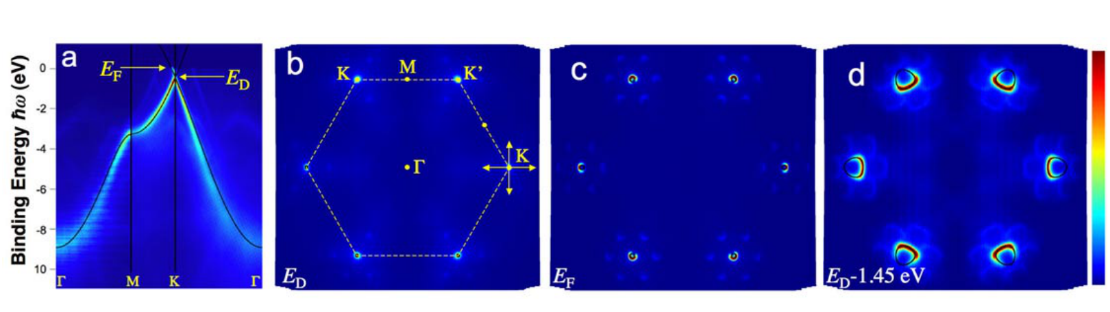
Figure adapted from Bostwick et al., Nature Physics 3, 36 (2007), Fig. 1.

Challenge 1#

In the limit of having the exact exchange-correlation functional, should you expect KS-DFT orbital energies to deliver exact band structures?
Discuss among the group and be ready to share your thoughts with the class.

Band structures: Graphene#

Build system and solve SCF#

atoms = Graphene('C', latticeconstant={'a':2.46, 'c': 7})
atoms.calc = QEpyCalculator(qe_options=qe_options, logfile='tmp.out')
energy = atoms.get_potential_energy()

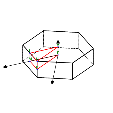
Look at the FBZ and select special \(k\) points#

lat = atoms.cell.get_bravais_lattice()
lat.plot_bz(show=True)

_images/2f730eca6d34b70e949ed560ce8b7dcc42a4811c6abc13b35c7b29681e60d310.png

<Axes3D: >

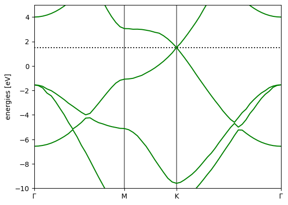
Choose \(\Gamma \to M \to K \to \Gamma\) band path#

Plot the first 6 bands#

path = atoms.cell.bandpath('GMKG',npoints=61)
qe_options['&system']['nbnd']=8
band = atoms.calc.get_band_structure(qe_options, kpts=path)#, reference=atoms.calc.get_fermi_level())
band.subtract_reference()
band.plot()

<Axes: ylabel='energies [eV]'>

_images/18d55c7f9e7a7a6f9e0014ceca9370e003149b4eb9ac7695f2c5622efb81686c.png

Challenge 1.2#

Band structure of Si diamond structure
Use the hands-on band structure tutorial. Notice the ASE tool Bulk from ase.build

from ase.build import bulk
atoms = bulk('Si','diamond',a=5.431)

Compare the notebook for Si and for graphene
Make a new notebook with a system of your choice and compute the band structure.

PART II: TDDFT based on KS-DFT#

Electronic excitations and UV–vis spectroscopy#

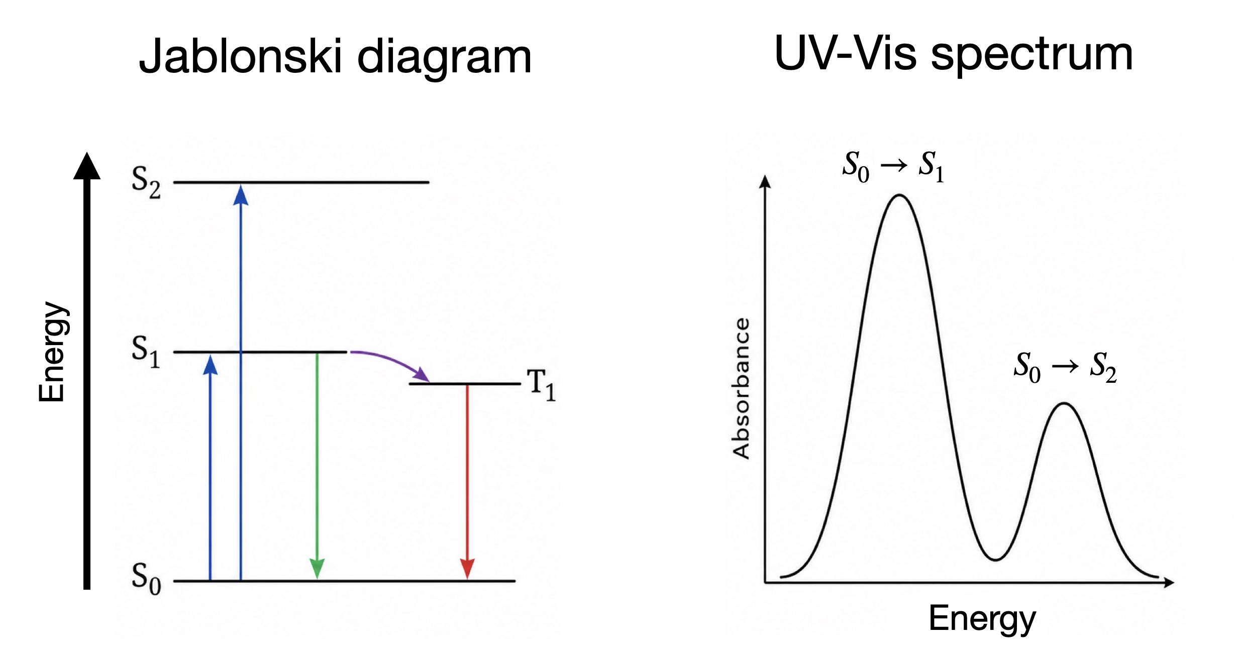
UV–vis absorption probes electronic excitations from the ground singlet \(S_0\) to excited singlets \(S_n\) at photon energy \(E = h\nu\).
In a Jablonski diagram, upward arrows are absorption; downward arrows are fluorescence; wavy/dashed paths are internal conversion and intersystem crossing.
Each allowed \(S_0 \to S_n\) transition contributes a peak in the spectrum.

TDDFT vs experiment: \(S_0 \to S_1\) excitation energies#

Benchmark on 29 small molecules: mean absolute error (MAE) of \(S_0 \to S_1\) excitations vs experiment.
Wavefunction methods vs TD-DFT functionals.

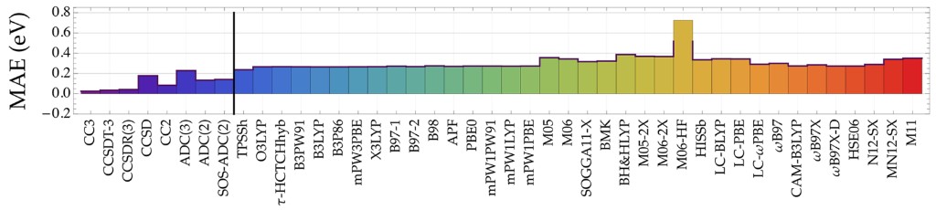
Adapted from Suellen et al., J. Chem. Theory Comput. 15, 4581 (2019), Fig. 3 (doi:10.1021/acs.jctc.9b00446).

Let’s dive a bit deeper into TDDFT#

Real-time TDDFT equations :#

\[ -\frac{1}{2}\nabla^2 \phi_k(\mathbf{r},t) + \color{red}{v_s(\mathbf{r},t)}\,\phi_k(\mathbf{r},t) = i\,\frac{\partial \phi_k(\mathbf{r},t)}{\partial t} \]

\[ n(\mathbf{r},t) = \sum_k f_k\, \lvert \phi_k(\mathbf{r},t) \rvert^2, \qquad N = \sum_k f_k, \quad \text{with } \{f_k\} \text{ time-independent.} \]

The rt-TDDFT equations can be integrated in time#

This approach delivers \(\{\phi_k(\mathbf{r},t)\}\) and thus \(n(\mathbf{r},t)\)

…and any other derived quantity

ultrafast electron dynamics (scattering, Coulomb explosions, stopping power, etc…)

electronic oscillations in the frequency domain, \(n(\mathbf{r},\omega)=\int n(\mathbf{r},t)\, e^{i\omega t}\, dt\), give access to spectra

Why does \(n(\mathbf{r},\omega)\) yield spectra?#

Out of equilibrium, the time-dependent wavefunction could be

\[ |\Psi(t)\rangle = c_0 e^{-iE_0t/\hbar}|\Psi_0\rangle + c_1 e^{-iE_1t/\hbar}|\Psi_1\rangle . \]

The corresponding time-dependent density is

\[ n(\mathbf r,t) = \langle \Psi(t)|\hat n(\mathbf r)|\Psi(t)\rangle =\underbrace{|c_0|^2n_0(\mathbf r)+|c_1|^2n_1(\mathbf r)}_{n(\mathbf{r},t=0)} + \underbrace{c_0^*c_1 n_{01}(\mathbf{r}) e^{-i(E_1-E_0)t/\hbar}+ c_1^*c_0 n_{10}(\mathbf{r})e^{i(E_1-E_0)t/\hbar}}_{\delta n(\mathbf{r},t)} \]

\(\delta n(\mathbf{r},t)\) oscillates at the excitation frequency \(\omega_{01} = \frac{E_1-E_0}{\hbar},\) with amplitude given by the transition density \(n_{10}(\mathbf r) = n_{01}(\mathbf r)=\langle \Psi_0|\hat n(\mathbf r)|\Psi_1\rangle\).

In the frequency domain, these oscillations produce peaks at the excitation energies:

\[ \delta n(\mathbf r,\omega) = c_0^*c_1 n_{01}(\mathbf r)\, \delta(\omega-\omega_{01}) \color{grey}{+c_0c_1^* n_{10}(\mathbf r)\, \delta(\omega+\omega_{01})} \]

Therefore, the frequencies contained in \(\delta n(\mathbf r,\omega)\) give access to the excitation spectrum.

Two important ingredients of TDDFT#

#1: The occupation numbers#

\[ n(\mathbf{r},t) = \sum_k f_k\, \lvert \phi_k(\mathbf{r},t) \rvert^2, \qquad N = \sum_k f_k, \quad \text{with } \{f_k\} \text{ time-independent.} \]

Challenge 2#

The occupation numbers, \(\{f_k\}\), are taken to be independent of time. Why?

Discuss among the group and be ready to share your thoughts with the class.

#2: The time-dependent KS potential#

\[ v_s(\mathbf{r},t) = v_H(\mathbf{r},t) + v_{ext}(\mathbf{r},t) + \color{red}{v_{xc}(\mathbf{r},t)} \]

is defined as that particular potential such that \(n_{KS}(\mathbf{r},t) = n(\mathbf{r},t)\)

Once \(v_{xc}(\mathbf{r},t)\) is approximated, we can integrate the rt-TDDFT equations

Several software implement rt-TDDFT, and if time permits, we will consider it later in this lecture

Challenge 3#

How can \(v_{xc}(\mathbf{r},t)\) be approximated? Would \(v_{xc}(\mathbf{r},t)= v_{xc}[n(t)](\mathbf{r}) = \frac{\delta E_{xc}[n]}{\delta n(\mathbf{r})}\bigg\vert_{n=n(\mathbf{r},t)}\) be a good approximation?

Discuss among the group and be ready to share your thoughts with the class.

The adiabatic approximation in rt-TDDFT#

\[ v_{xc}(\mathbf{r},t) = v_{xc}[n(t)](\mathbf{r}) \]

uses the ground state XC functional and potential and evaluates them with the time-dependent density, \(n(\mathbf{r},t)\).

The time-dependent xc potential is not defined in this way

The adiabatic approximation is perhaps the best we can do. But together with the self-interaction error, it leads to some shortcomings:
- charge-transfer excitations are generally too low in energy
- predicted optical gaps are usually too low (e.g., PBE water: 6.5 eV vs 8.5 eV, see also this paper.)
- neglect of double excitations (e.g., 1,3-butene)

There are fixes but you must evaluate them carfully before use.
- use of hybrids
- use of GGA+U
- use of long-range corrected xc potentials (LB94, SAOP)
- other functionals (Koopman’s, etc)

Does \(v_{xc}(\mathbf{r},t)\) exist?#

The KS-TDDFT equations are the result of the Runge-Gross theorem, the follow-up van Leuwen theorem and considerations by Vignale.

Targeting the excited states directly: linear-response TDDFT#

Idea: consider small variations, \(\delta v_{\mathrm{appl}}\), of the external potential

In other words:#

The lr-TDDFT equations define variations \(\longleftrightarrow\) response relations as

\[ \color{green}{\text{Int: }} v_{ext}(\mathbf{r},t) - v_{ext}(\mathbf{r},0)=\color{green}{\delta v_{appl}(\mathbf{r},t) \longleftrightarrow \delta n(\mathbf{r},t)}=n(\mathbf{r},t) - n(\mathbf{r},0) \]

\[ ~~~~~~~~\color{red}{\text{KS: }}~v_s(\mathbf{r},t) - v_s(\mathbf{r},0)=\color{red}{\delta v_s(\mathbf{r},t) \longleftrightarrow \delta n(\mathbf{r},t)} = n(\mathbf{r},t) - n(\mathbf{r},0) \]

and in frequency domain:

\[ \color{green}{\delta v_{appl}(\mathbf{r},\omega) \longleftrightarrow \delta n(\mathbf{r},\omega)} \qquad \color{red}{\delta v_s(\mathbf{r},\omega) \longleftrightarrow \delta n(\mathbf{r},\omega)} \]

We now express these relations in the limit of linear response

Linear density response of the interacting system#

For a weak perturbing potential \(\delta v_{\mathrm{appl}}(\mathbf{r},\omega)\), the density response, \(\delta n(\mathbf{r},\omega)\), satisfies

\[ \delta n(\mathbf{r},\omega) = \int \chi(\mathbf{r},\mathbf{r}',\omega)\, \delta v_{\mathrm{appl}}(\mathbf{r}',\omega)\, d\mathbf{r}' ~~ \color{green}{\longleftrightarrow} ~~ \chi(\mathbf{r},\mathbf{r}',\omega) = \frac{\delta n(\mathbf{r},\omega)}{\delta v_{\mathrm{appl}}(\mathbf{r}',\omega)}~~~~~~~~~~ \]

where \(\chi\) is the density response function of the interacting system

Does \(\delta n = \chi\,\delta v_{\mathrm{appl}}\) make sense to you?

Why is \(\chi\) interesting?#

From first-order perturbation theory, it can be shown that:

\[ \chi(\mathbf r,\mathbf r',\omega) = \sum_{k\neq 0} \left[ \frac{ n_{0k}(\mathbf r)\,n_{k0}(\mathbf r') }{ \omega-\Omega_{0k}+i\eta } - \frac{ n_{k0}(\mathbf r)\,n_{0k}(\mathbf r') }{ \omega+\Omega_{0k}+i\eta } \right] \]

\[ \chi_s(\mathbf r,\mathbf r',\omega) = \sum_{i\in\mathrm{occ}} \sum_{a\in\mathrm{vir}} \frac{ \phi_i(\mathbf r)\phi_a(\mathbf r)\, \phi_i(\mathbf r')\phi_a(\mathbf r') }{ \omega-\omega_{ia}-i\eta } +\mathrm{c.c.}, \qquad \omega_{ia} = \frac{\varepsilon_a-\varepsilon_i}{\hbar} \]

Linear density response of the KS system#

To find \(\chi\) we once again consider the Kohn–Sham non-interacting system.

The interacting and KS systems bust share the same density reponse, \(\delta n\) (using a short-hand notation)

\({\color{red}\chi}\,\delta v_{\mathrm{appl}}\)

\(\chi_s\,{\color{red}\delta v_s}\)

In red the quantities unknown.

The above is true for a special \(\delta v_s\) such that the induced density variations, \(\delta n\), of the interacting and KS systems are equal.

What is \(\color{red}{\delta v_s}\)?#

\[ \delta v_s(\mathbf{r},\omega) = \delta v_H(\mathbf{r},\omega) + \color{red}{\delta v_{\mathrm{xc}}(\mathbf{r},\omega)} + \delta v_{\mathrm{appl}}(\mathbf{r},\omega) \]

where \(\delta v_H(\mathbf{r},\omega) = \int \dfrac{\delta n(\mathbf{r}',\omega)}{|\mathbf{r}-\mathbf{r}'|}\, d\mathbf{r}'\) and \(\delta v_{xc}(\mathbf{r},\omega) = \int d\mathbf{r}' f_{\mathrm{xc}}(\mathbf{r},\mathbf{r}',\omega)\,\delta n(\mathbf{r}'\omega)\), defining an xc kernel.

Combining the definitions introduced thus far (using a short-hand notation):

\[ \chi \delta v_{appl} = \chi_s \delta v_{appl} + \chi_s \bigg(\frac{1}{|\mathbf{r}-\mathbf{r}'|}+f_{xc}(\mathbf{r},\mathbf{r}',\omega)\bigg)\delta n \]

By taking the derivative with respect to \(\delta v_{\mathrm{appl}}\), we obtain the important Dyson-like relation:

\[ \chi = \chi_s + \chi_s f_{\mathrm{Hxc}} \chi \]

Casida equations#

The inverse of the Dyson equation is

\[ -\chi^{-1} = -\chi_s^{-1} + f_{Hxc}(\mathbf{r},\mathbf{r}',\omega) \]

can be expressed in a basis set of occupied/virtual products, leading to the Casida equation

\[\begin{split} \begin{pmatrix} {\bf A}(\omega) & {\bf B}(\omega) \\ {\bf B}(\omega) & {\bf A}(\omega) \end{pmatrix} \begin{pmatrix} X_{ia} \\ Y_{ia} \end{pmatrix} = \omega \begin{pmatrix} 1 & 0 \\ 0 & -1 \end{pmatrix} \begin{pmatrix} X_{ia} \\ Y_{ia} \end{pmatrix} \end{split}\]

where

\[ A_{iajb}(\omega) = \delta_{ij}\delta_{ab}\,\omega_{ia} + \big\langle \phi_i \phi_a \big| f_{Hxc}(\mathbf{r},\mathbf{r}',\omega) \big| \phi_j \phi_b \big\rangle, \qquad B_{iajb}(\omega) = \big\langle \phi_i \phi_a \big| f_{Hxc}(\mathbf{r},\mathbf{r}',\omega) \big| \phi_j \phi_b \big\rangle \]

with \(\omega_{ia} = \varepsilon_a - \varepsilon_i\), are the KS orbital excitations.

Excitation energies \(\Omega_k\) and the eigenvectors \((X_{ia}, Y_{ia})\) deliver transition densities \(n_{0k}(\mathbf{r}) = \sum_{ia} (X_{ia}+Y_{ia})\phi_i(\mathbf{r})\phi_a(\mathbf{r})\).

What can you obtain from lr-TDDFT?#

excitation energies / spectra
check out this nice paper

transition densities, transition dipoles and other derived quantities

e-e structure factors, dielectric functions, etc…
you’ll learn about some of these applications next week

Ready for some hands-on work?#