DFT introduction #3 (short lecture)
Team Rutgers(Michele, Ezekiel & Valeria)Rutgers University-Newark |
 |
| An interactive session |
Retrieve this presentation at:
mini ASESMA 2026 \(\bullet\) Accra, Ghana \(\bullet\) June 17, 2026
Goal of this lecture#
Understand occupations (aufbau and smearing)
Understand and code the Self-Consistent Cycle (SCF)
Band structure / DOS
Split into N groups#
Assign number
1-Nto each studentGroups sit together
Possibly have 1 instructor per group
The KS equations#
In discretized form#
How can we solve it?#
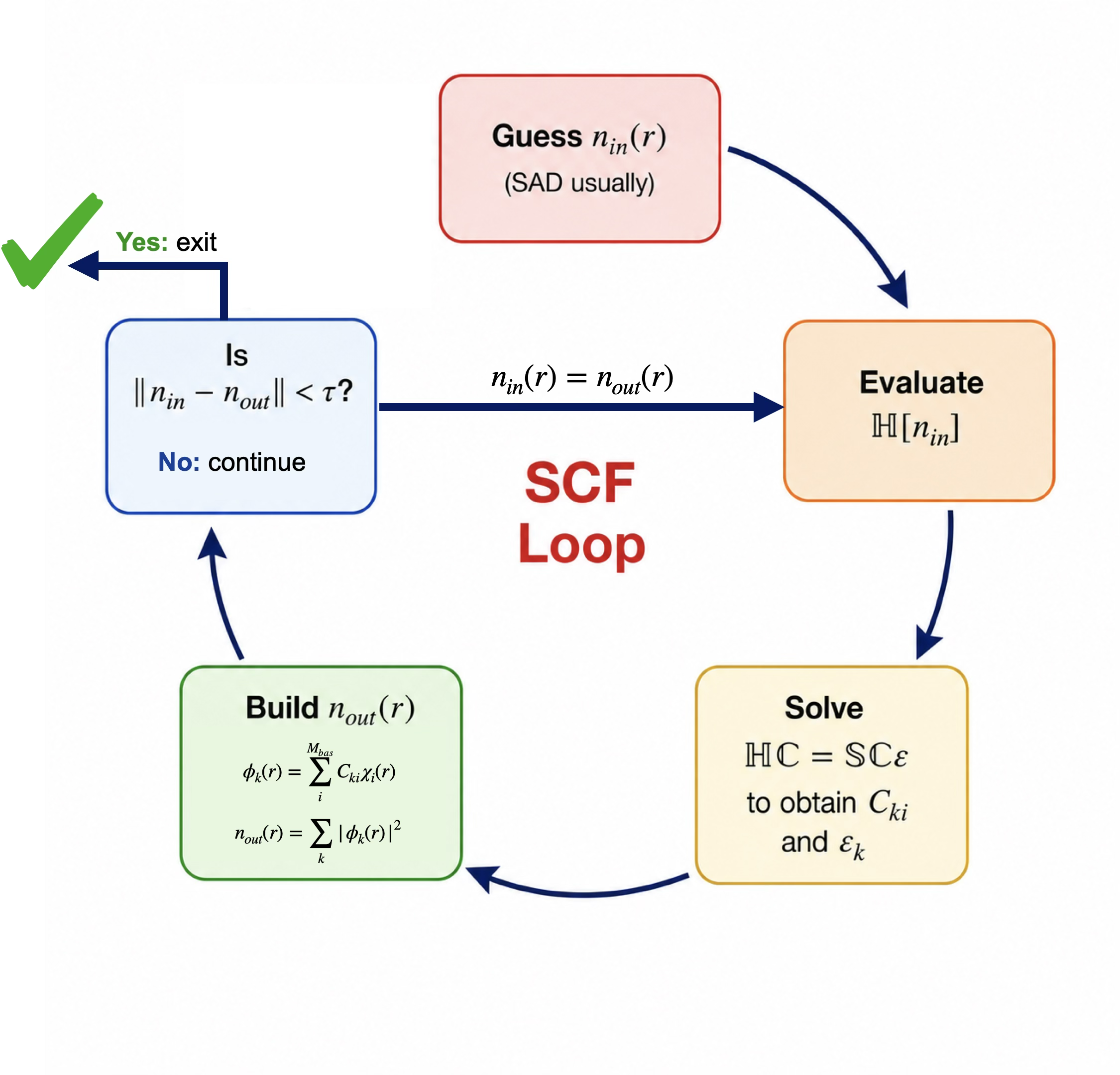
\(\mathbb{H}\) depends on \(v_s(r)\) which depends on \(n(r)\)#
uniform density
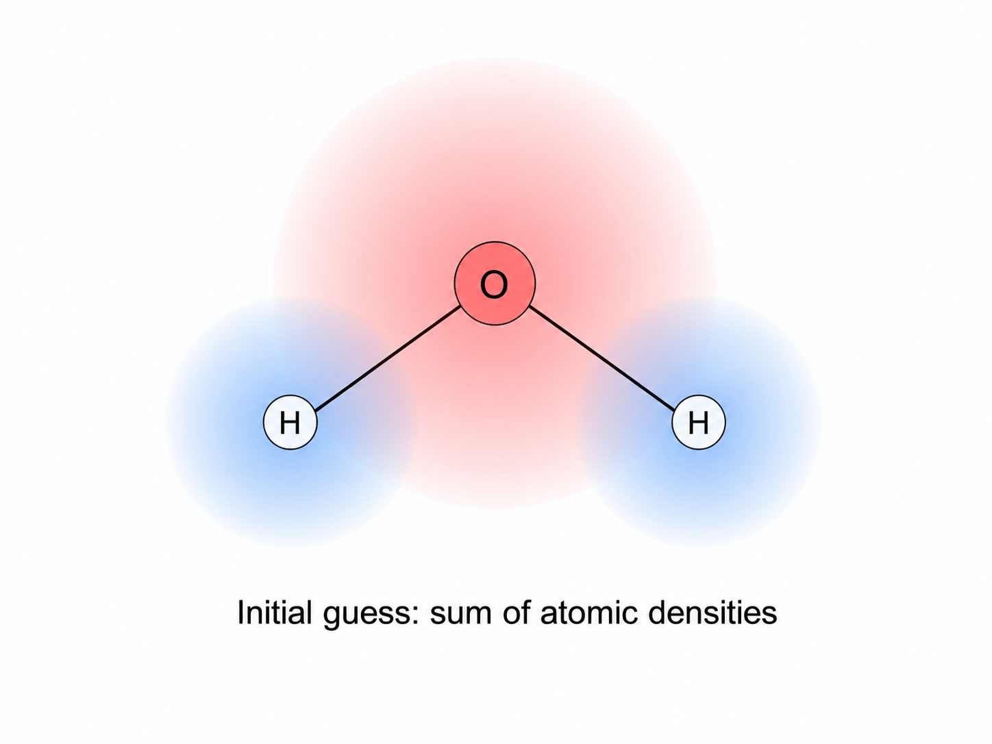
sum of atomic densities (SAD), usually taken from the pseudopotential
The Self-Consistent Field (SCF) loop#
In QEpy and QE, the SCF is a basic workflow#
QE handles it via the card
&control
QEpy via the equivalent card in the options dictionary, like this:
qe_options = {}
qe_options['&control'] = {}
qe_options['&control']['calculation'] = 'scf'
The SCF threshold#
\(\tau\) usually is in units of energy. Appropriate convergence conditions are
Challenge 1#
The electron density
Derive the equation for obtaining the electron density from the basis functions \(\{\chi_k(r)\}\) and the wavefunction coefficients \(\{C_{ki}\}\). Use the expression

Occupation numbers#
The usual equation (remember (N) is the number of electrons):
For nonzero \(T\), or for small gaps \(\left(E_g \ll 1\right)\), where the SCF procedure may have difficulty converging:
For solids, the need for (k)-point sampling often requires smearing:
Challenge 2: what are these \(f_k\)?#
Code your own Fermi-Dirac smearing function to generate occupation numbers \(\{f_k\}\) given orbital energies \(\{\varepsilon_k\}\)
Consider a set of eigenvalues, \(\{\varepsilon_k\}\) coming from \(\color{green}{\mathbb{HC}=\mathbb{SC\varepsilon}}\). Evaluate the Fermi-Dirac distribution and impose \(\sum_k f_k = N\). Feel free to use AI to help you code it. Justify and explain your code to a tutor.
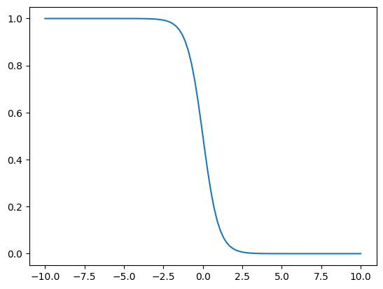
import matplotlib.pyplot as plt
import numpy as np
x=np.linspace(start=-10,stop=10,num=100)
tau = 0.5
plt.plot(x,(1+np.exp((x-0)/tau))**(-1))
[<matplotlib.lines.Line2D at 0x138595a50>]